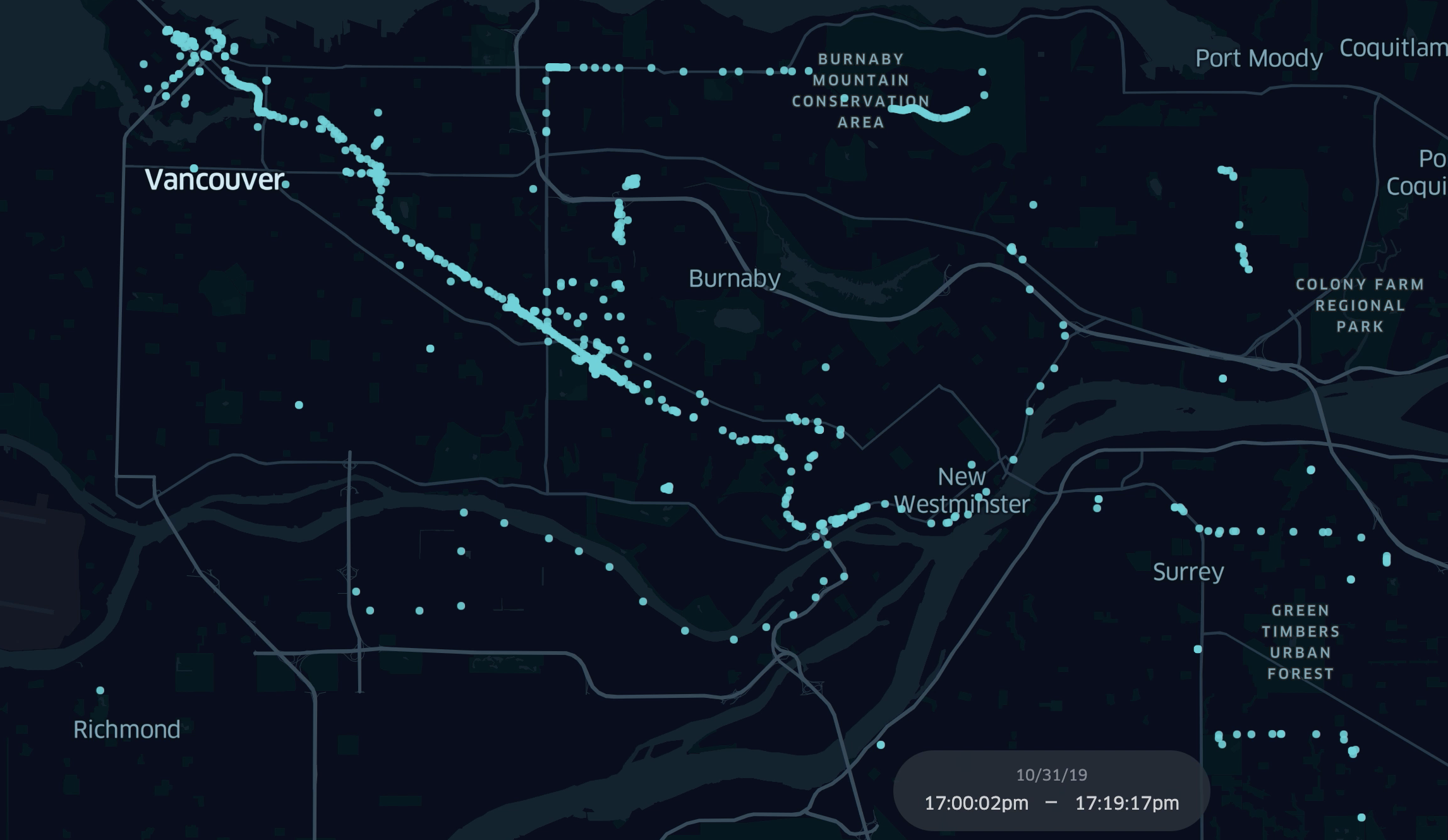
(Note: this is adapted from my talk at 2021 Scale by the Bay, Location-Based Data Engineering for Good)
If you are a data scientist, chances are you are coding Python and most likely using pandas. You might have heard of or are learning Apache Spark, as while pandas on your laptop can last you for a good while -- eventually, you need to play with more data. Spark is perhaps the best-known big data tool, and as you'd like to get up to speed as quickly as possible, you pick up PySpark, Spark's Python API for data processing at scale. Good choice!
(I'm probably biased, but if you really want to be a Spark expert, you should absolutely learn Scala. That will let you get the full power of all of Spark's APIs, as well as extend Spark in any way possible.
You will also probably learn some awesome concepts along the way, such as functional programming.)
In this article, I'm going to focus on PySpark's windowing operations. Windowing operations let you use data from adjacent rows, enabling the easy tackling of some nontrivial data processing that typically involves sessions or custom code. I will use an example from location-based data processing.
Example: Traffic Analysis from Mobile Data

I'm going to use an interesting example from trip and traffic analysis of mobile location data. Apps that display ads and cell phones often give off data about locations very frequently. The data contains fields for mobility analysis such as device ID, timestamp, and location information:
+--------------------+----------+----------+------------+
|            deviceID| timestamp|  latitude|   longitude|
+--------------------+----------+----------+------------+
|0000606e153fb72d5...|1562010606|     37.17|   -104.7348|
|00043157f6342b342...|1562020544| 37.050922|  -104.78587|
|00043157f6342b342...|1562021967|  37.05095|  -104.78588|
|00043157f6342b342...|1562021161| 37.050922|  -104.78587|
|00043157f6342b342...|1562019848| 37.050922|  -104.78587|
|00048d7fb00ee2961...|1561941291|37.2118654|-104.9377987|
|00048d7fb00ee2961...|1561953983|37.2118649|-104.9379102|
If we process this data into trips with origins and destinations summarized, it could be used by, for example, city planning departments:
Where do people who visit city parks come from, and how do they visit?
How can we plan and locate parks and recreational facilities to maximize accessibility for everyone?
Do people always go to the closest amenity? If not, why?
How can public transit routes be improved?
A data science workflow to transform this raw mobility data into trips and origin/destination data for analysis might involve these steps:
Normalize and sessionize (sort by device ID)
Coalesce events in similar locations to a single event with
countUse inference/ML to determine which events may be an origin/destination
Coalesce and sort O/D pairs into trips
Sessionizing by Device ID
Sessionizing or grouping events by device is fairly trivial in PySpark. Spark can easily read subdirectory trees straight from Azure / AWS / GCS / etc. containing hundreds of files:
    df = spark.read.parquet("wasbs://container1@blah.blob.core.windows.net/xx/yy/zz/2020/01")
    return df.select(
        [
            col("advertiser_id").alias("deviceID"),
            col("location_at").alias("timestamp"),
            col("latitude"),
            col("longitude"),
        ]
    )
Sorting many GBs or TBs of data by device ID to sessionize - no problem!
return df.sort("deviceID")
Note that the capability to read directory trees with many files and sort a huge amount of data trivially seems like table stakes for any big data framework, but this Spark capability is very difficult to do with just Python and pandas -- and this illustrates a major differentiator with frameworks like Spark.
Avoiding custom Python processing code
One key initial processing step involves grouping or collapsing successive points that are in the "same" location into a single "event" with a count and start/end time. This lets us determine the periods during which a device remained stationary. The person is probably at home or in the office, or restaurant, or somewhere where they will stay for a while. This information is crucial for trip and origin/destination inference.
In order to collapse successive mobile pings, we find the distance between the lat and long of successive points. We could use simple hypotenuse, although we could also use proper geospatial math libraries to compute ground/air distance.
In Python, one might accomplish this by iterating over each row, tracking the previous row's lat and long, then using a simple calculation based on the saved state to compute the distance.
    def process(df):
        for row in range(1, len(df)):
            if prevlat and prevDevice == df[row]["deviceID"]:
                dist = hypot(df[row]["latitude"] - prevlat,
                             df[row]["longitude"] - prevlong)
                prevlat = df[row]["latitude"]
                prevlong = df[row]["longitude"]
                df[row]["distance"] = dist
Could you do the same thing in pySpark?
Well, you could, but you wouldn't want to. It would be very slow.
You see, when you do a simple operation such as a df.sort(), what PySpark does under the hood is translate the Python call into a query execution plan, which contains a primitive, a command if you will, to sort the dataframe. When Spark executes the operation, it looks at the plan and carries out the sort operation in a distributed way. On each Spark node, the work is carried out in native JVM compiled bytecode, very very fast. None of the work happens in the Python interpreter.
On the other hand, if we were to ask PySpark to execute the code inside process() manually, Spark would have to do the following:
Ship the Python code and dependencies out to all nodes
Translate the data from Spark's native in-memory dataframe format (or from source) to a format Python/pandas can understand
Invoke the Python interpreter, in a separate process, and send it the dataframe data
Call Python and the function above to process the data
Get the data back from the Python process and translate the results back into Spark's native format
The extra cost of the relay would be expensive, and running the custom code in Python would be slower than Spark could natively execute it as well. In addition, the iterative code above has to get boundary conditions such as different deviceIDs correct, which is often easy to get wrong.
The solution is to use a set of native functions in PySpark that we call the windowing functions. They let us operate on data in adjacent rows in a way native to Spark execution.
PySpark Windowing Functions 101
The windowing functions operate on a sliding window over the current dataset, centered around a current row. Two of the fundamental windowing functions are lag (previous) and lead (next) for row lookup.
| Lag | Indx | deviceID | timestamp | latitude | longitude |
| Lag | -5 | 0000606e153fb72d5... | 1562010606 | 37.17 | -104.7348 |
| Lag | -4 | 00043157f6342b342... | 1562020544 | 37.050922 | -104.78587 |
| Lag | -3 | 00043157f6342b342... | 1562021967 | 37.05095 | -104.78588 |
| Lag | -2 | 00043157f6342b342... | 1562021161 | 37.050922 | -104.78587 |
| Lag | -1 | 00043157f6342b342... | 1562019848 | 37.050922 | -104.78587 |
| Cur | 0 | 00048d7fb00ee2961... | 1561941291 | 37.2118654 | -104.9377987 |
| Lead | 1 | 00048d7fb00ee2961... | 1561953983 | 37.2118649 | -104.9379102 |
| Lead | 2 | 00048d7fb00ee2961... | 1561974623 | 37.2118598 | -104.9378926 |
| Lead | 3 | 00048d7fb00ee2961... | 1561948360 | 37.2118591 | -104.9379316 |
For example, the following uses the lag function to look up the lat and lon from the previous row to compute hypotenuse distance:
>>> w = Window.partitionBy("deviceID").orderBy("timestamp")
>>> df1 = df.withColumn("dist_from_prev",
...   F.hypot(F.col("latitude") - F.lag("latitude", 1).over(w),
...           F.col("longitude") - F.lag("longitude", 1).over(w)))
>>> df1.show(30)
This yields the following output:
+--------------------+----------+----------+------------+--------------------+
|            deviceID| timestamp|  latitude|   longitude|      dist_from_prev|
+--------------------+----------+----------+------------+--------------------+
|0000606e153fb72d5...|1562010606|     37.17|   -104.7348|                null|
|00043157f6342b342...|1562019848| 37.050922|  -104.78587|                null|
|00043157f6342b342...|1562020544| 37.050922|  -104.78587|                 0.0|
|00043157f6342b342...|1562021161| 37.050922|  -104.78587|                 0.0|
|00043157f6342b342...|1562021967|  37.05095|  -104.78588|2.973213749604462...|
|00048d7fb00ee2961...|1561939554|37.2647663|-105.0801919|                null|
|00048d7fb00ee2961...|1561939974|37.2693613|-105.0483915| 0.03213066238284813|
The above is very succinct, and PySpark is able to translate the above into a highly optimized physical plan. Win-win!
Defining the PySpark Window
You might have noticed the Window.partitionBy above. This is important - PySpark is able to partition the input dataset by a field. What this means is that the window above only contains data from a single deviceID - PySpark partitions your input data by the field given in the partitionBy clause. If for example we are at the second row in the input data above, which is the first row for deviceID 0004315..., then the window would start from that row and go forwards. This is super useful, since it would make no sense to compute the distance using a previous row which did not belong to the same deviceID!
PySpark will also keep data sorted by timestamp in this case within each partition.
The combination of partitionBy() and orderBy() is very very useful for sessionizing data here and processing with window functions.
Coalescing Similar Locations
Now, let's use some more windowing functions to achieve our goal of coalescing successive pings which are at the "same" location. First, we want to identify the "first" and "last" rows of a "group" of pings at similar locations, or where the distance is below a certain delta:
    # True == this is first row of movement.  False == moved < delta from last location
    df1 = df1.withColumn(
        "first_row",
        when(
            F.isnull(col("dist_from_prev")) | (col("dist_from_prev") > delta), True
        ).otherwise(False),
    )

    # Also add a last_row column, which is true if this is the last row of a group at the same location
    # (or the last row of a deviceID).  We use a trick - the lead windowing function lets us peek _ahead_!
    df1 = df1.withColumn("last_row", F.lead("first_row", 1, default=True).over(w))
Note the use of the F.lead() function to look ahead of the current row... this works even though "first row" needs to be computed too! The output:
| deviceID | timestamp | latitude | longitude | dist_from_prev | first_row | last_row |
| 00606e153fb72d5... | 1562010606 | 37.17 | -104.7348 | null | true | true |
| 043157f6342b342... | 1562019848 | 37.050922 | -104.78587 | null | true | false |
| 043157f6342b342... | 1562020544 | 37.050922 | -104.78587 | 0.0 | false | false |
| 043157f6342b342... | 1562021161 | 37.050922 | -104.78587 | 0.0 | false | false |
| 043157f6342b342... | 1562021967 | 37.05095 | -104.78588 | 2.973213749604462 | false | true |
| 048d7fb00ee2961... | 1561939554 | 37.2647663 | -105.0801919 | null | true | true |
| 048d7fb00ee2961... | 1561939974 | 37.2693613 | -105.0483915 | 0.03213066238284 | true | true |
| 048d7fb00ee2961... | 1561940425 | 37.2520333 | -104.9769234 | 0.07353875781931 | true | true |
Next, we add a count to the "last row".
We annotate row numbers for rows that are "first rows", then use the last() function to find the last row with a row number, and the count is the difference in row numbers:
df1 = df1.withColumn("start_row_tmp", when(col('first_row') == True,
                                           F.row_number().over(w)))
df1 = df1.withColumn("count", when(col('last_row') == True,
            F.row_number().over(w) -
            F.last('start_row_tmp', ignorenulls=True).over(
                  w.rowsBetween(Window.unboundedPreceding, 0)) + 1))
| deviceID | timestamp | latitude | longitude | first_row | last_row | start_row_tmp | count |
| 00606e153fb72d5. | 1562010606 | 37.17 | -104.7348 | true | true | 1 | 1 |
| 043157f6342b342. | 1562019848 | 37.050922 | -104.78587 | true | false | 1 | null |
| 043157f6342b342. | 1562020544 | 37.050922 | -104.78587 | false | false | null | null |
| 043157f6342b342. | 1562021161 | 37.050922 | -104.78587 | false | false | null | null |
| 043157f6342b342. | 1562021967 | 37.05095 | -104.78588 | false | true | null | 4 |
| 048d7fb00ee2961. | 1561939554 | 37.2647663 | -105.0801919 | true | true | 1 | 1 |
| 048d7fb00ee2961. | 1561939974 | 37.2693613 | -105.0483915 | true | true | 2 | 1 |
| 048d7fb00ee2961. | 1561940425 | 37.2520333 | -104.9769234 | true | true | 3 | 1 |
Then you just filter for the last row, and boom we have coalescing!
Where to Go From Here
To learn more, have a look at the PySpark docs for windowing functions, or have a look at SQL Window functions from which the PySpark functions drew their inspiration.
Happy data crunching!

